Query Zoo: DSL Gallery for Multilayer Analysis

The Query Zoo is a curated gallery of DSL queries that demonstrate the expressiveness and power of py3plex for multilayer network analysis.

Each example:

• Solves a real multilayer analysis problem

• Uses the DSL end-to-end with idiomatic patterns

• Produces concrete, reproducible outputs

• Is fully tested and documented

Why a Query Zoo?

The DSL is most powerful when you see it in action on realistic problems. This gallery shows you how to think about multilayer queries, not just what the syntax is. Use these examples as recipes and starting points for your own analyses.

Overview

The Query Zoo is organized around common multilayer analysis tasks:

1. Basic Multilayer Exploration — Understand layer statistics and structure

2. Cross-Layer Hubs — Find nodes that are important across multiple layers

3. Layer Similarity — Measure structural alignment between layers

4. Community Structure — Detect and analyze multilayer communities

5. Multiplex PageRank — Compute multilayer-aware centrality

6. Robustness Analysis — Assess network resilience to layer failures

7. Advanced Centrality Comparison — Identify versatile vs specialized hubs

8. Edge Grouping and Coverage — Analyze edges across layer pairs with top-k and coverage

9. Layer Algebra Filtering — Use layer set algebra for flexible layer selection

10. Cross-Layer Paths with Algebra — Find paths while excluding certain layers

11. Null Model Comparison — Statistical significance testing against null models

12. Bootstrap Confidence Intervals — Estimate uncertainty in centrality measures

13. Uncertainty-Aware Ranking — Rank nodes considering variability across layers

All examples use small, reproducible multilayer networks from the examples/dsl_query_zoo/datasets.py module with fixed seeds so you can match the outputs shown here.

Tip

Running the Examples

All query functions are available in examples/dsl_query_zoo/queries.py. To run all queries and generate outputs:

python examples/dsl_query_zoo/run_all.py

Test the queries with:

pytest tests/test_dsl_query_zoo.py

---

1. Basic Multilayer Exploration

Problem: You’ve loaded a multilayer network and want to quickly understand its structure. Which layers are densest? How many nodes and edges does each layer have?

Solution: Compute basic statistics per layer using the DSL.

Query Code

def query_basic_exploration(network: Network) -> pd.DataFrame:
    """Summarize layers: node counts, edge counts, and average degree per layer.

    Refactored: single DSL query over all layers + pandas groupby, no explicit
    for-loop over layers.

    This query demonstrates basic multilayer exploration by computing
    fundamental statistics for each layer independently. This is typically
    the first step in multilayer analysis to understand the structure
    and identify layers with different connectivity patterns.

    Why it's interesting:
    - Reveals which layers are denser or sparser
    - Identifies layers that might be hubs of activity
    - Shows structural diversity across the multilayer network

    DSL concepts demonstrated:
    - SELECT nodes from all layers in one shot
    - Computing degree per layer
    - Vectorized aggregation by layer

    Args:
        network: A multi_layer_network instance

    Returns:
        pd.DataFrame with columns: layer, n_nodes, n_edges, avg_degree
    """
    result = (
        Q.nodes()
         .from_layers(L["*"])       # all layers in one shot
         .compute("degree")
         .execute(network)
    )

    if len(result) == 0:
        return pd.DataFrame(columns=["layer", "n_nodes", "n_edges", "avg_degree"])

    df = result.to_pandas()

    # One row per (node, layer), so size() is node count
    stats = (
        df.groupby("layer")
          .agg(
              n_nodes=("id", "size"),
              total_degree=("degree", "sum"),
              avg_degree=("degree", "mean"),
          )
          .reset_index()
    )

    stats["n_edges"] = (stats["total_degree"] // 2).astype(int)
    stats["avg_degree"] = stats["avg_degree"].round(2)

    return stats[["layer", "n_nodes", "n_edges", "avg_degree"]]

Why It’s Interesting

• First step in any analysis — Before diving into complex queries, understand your data

• Reveals layer diversity — Different layers often have vastly different structures

• Identifies sparse vs dense layers — Helps decide which layers need special handling

Example Output

Running on the social_work_network (12 people across social/work/family layers):

Layer	Nodes	Edges	Avg Degree
social	12	11	1.83
work	11	9	1.64
family	11	6	1.09

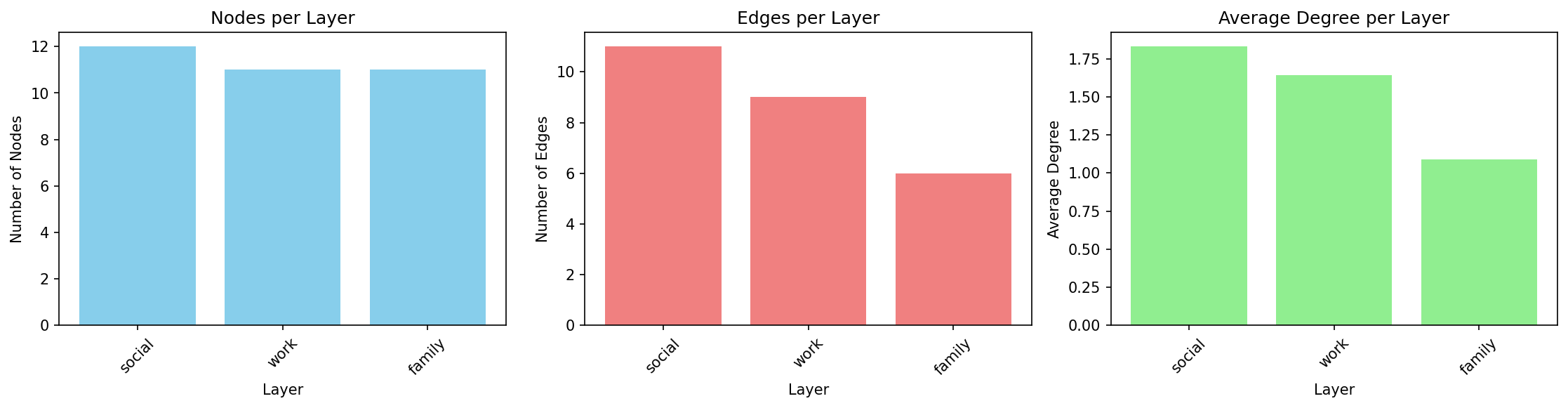
Interpretation: The social layer is densest (highest average degree), while family is sparsest. All layers have similar numbers of nodes, indicating good cross-layer coverage.

DSL Concepts Demonstrated

• Q.nodes().from_layers(L[name]) — Select nodes from a specific layer

• .compute("degree") — Add computed attributes to results

• .execute(network) — Run the query and get results

• .to_pandas() — Convert to DataFrame for analysis

---

2. Cross-Layer Hubs

Problem: Which nodes are consistently important across multiple layers? These “super hubs” are critical because they bridge different contexts.

Solution: Find top-k central nodes per layer, then identify which nodes appear in multiple layers’ top lists.

Query Code

def query_cross_layer_hubs(network: Network, k: int = 5) -> pd.DataFrame:
    """Find nodes that are consistently central across multiple layers.

    Refactored: one DSL query across all layers + pandas grouping, no explicit
    per-layer for loop.

    This query identifies "super hubs" - nodes that maintain high centrality
    across different layers. These nodes are particularly important because
    they serve as connectors across different contexts or domains.

    Why it's interesting:
    - Reveals nodes with consistent importance across contexts
    - Useful for identifying key actors in multiplex social networks
    - Helps understand cross-layer influence and information flow

    DSL concepts demonstrated:
    - Single query across all layers
    - Computing betweenness centrality
    - Vectorized top-k selection per layer using groupby
    - Coverage analysis (nodes appearing in multiple layers)

    Args:
        network: A multi_layer_network instance
        k: Number of top nodes to select per layer

    Returns:
        pd.DataFrame with nodes and their centrality scores per layer
    """
    result = (
        Q.nodes()
         .from_layers(L["*"])
         .compute("betweenness_centrality", "degree")
         .execute(network)
    )

    if len(result) == 0:
        return pd.DataFrame()

    df = result.to_pandas().rename(columns={"id": "node"})

    # Top-k by betweenness within each layer (vectorized)
    df_sorted = df.sort_values(["layer", "betweenness_centrality"],
                               ascending=[True, False])
    topk = df_sorted.groupby("layer").head(k)

    # Count how many layers each node appears in as a top-k hub
    coverage = (
        topk.groupby("node")["layer"]
            .nunique()
            .reset_index(name="layer_count")
    )

    result_df = (
        topk.merge(coverage, on="node")
            .sort_values(["layer_count", "betweenness_centrality"],
                         ascending=[False, False])
    )

    return result_df[["node", "layer", "degree",
                      "betweenness_centrality", "layer_count"]]

Why It’s Interesting

• Reveals cross-context influence — Nodes central in one layer might be peripheral in another

• Identifies key connectors — Nodes that appear in multiple layers’ top-k are especially important

• Robust hub detection — More reliable than single-layer centrality

Example Output

Top cross-layer hubs (k=5):

Node	Layer	Degree	Betweenness	Layer Count
Bob	social	3	0.0273	3
Bob	work	2	0.0	3
Bob	family	1	0.0	3
Alice	work	3	0.0889	2
Charlie	social	3	0.0273	2

Interpretation: Bob appears as a top-5 hub in all three layers (layer_count=3), making him the most versatile connector. Alice and Charlie are hubs in two layers each. layer_count is the number of distinct layers in which a node enters the per-layer top-k list.

DSL Concepts Demonstrated

• .compute("betweenness_centrality", "degree") — Compute multiple metrics at once

• .order_by("-betweenness_centrality") — Sort descending (- prefix)

• .limit(k) — Take top-k results

• Per-layer iteration and aggregation across layers

---

3. Layer Similarity

Problem: How similar are different layers structurally? Do they serve redundant or complementary roles?

Solution: Compute degree distributions per layer and measure pairwise correlations.

Query Code

def query_layer_similarity(network: Network) -> pd.DataFrame:
    """Compute structural similarity between layers based on degree distributions.

    Refactored: single DSL query + pivot, no explicit loops over layers/nodes.

    This query measures how similar different layers are in terms of their
    connectivity patterns. Layers with similar degree distributions likely
    serve similar structural roles in the multilayer network.

    Why it's interesting:
    - Identifies redundant or complementary layers
    - Helps understand layer specialization
    - Can inform layer aggregation or simplification decisions

    DSL concepts demonstrated:
    - Single query across all layers
    - Pivot table to create node × layer matrix
    - Correlation between layers via .corr()

    Args:
        network: A multi_layer_network instance

    Returns:
        pd.DataFrame: Pairwise correlation matrix of layer degree distributions
    """
    result = (
        Q.nodes()
         .from_layers(L["*"])
         .compute("degree")
         .execute(network)
    )

    if len(result) == 0:
        return pd.DataFrame()

    df = result.to_pandas()

    # Build node × layer degree matrix: rows = nodes, cols = layers
    degree_matrix = df.pivot_table(
        index="id",
        columns="layer",
        values="degree",
        fill_value=0,
    )

    # Correlation between columns = correlation between layers
    corr_df = degree_matrix.corr().round(3)

    # Optional: clean up index/column names for display
    corr_df.index.name = None
    corr_df.columns.name = None

    return corr_df

Why It’s Interesting

• Detects redundancy — High correlation suggests layers capture similar structure

• Guides simplification — Nearly identical layers might be merged

• Reveals specialization — Low/negative correlation shows layers serve different roles

Example Output

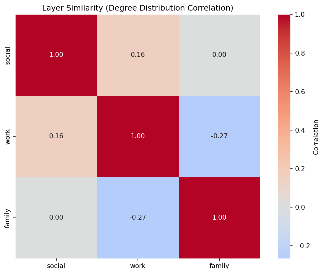
Correlation matrix for social_work_network:

	social	work	family
social	1.000	0.159	0.000
work	0.159	1.000	-0.267
family	0.000	-0.267	1.000

Interpretation: Social and work layers have weak positive correlation (0.159), suggesting some structural overlap. Family and work are negatively correlated (-0.267), indicating they capture different connectivity patterns. Correlations are Pearson coefficients computed from the node-by-layer degree matrix. Nodes missing from a layer contribute a degree of 0 in that matrix so every layer uses the same node ordering.

DSL Concepts Demonstrated

• Layer-by-layer degree computation

• Aggregating results across layers for meta-analysis

• Using computed attributes for layer-level comparisons

---

4. Community Structure

Problem: What communities exist in the multilayer network? How do they manifest across layers?

Solution: Detect communities using multilayer community detection, then analyze their distribution across layers.

Query Code

def query_community_structure(network: Network) -> pd.DataFrame:
    """Detect communities and analyze their distribution across layers.

    This query finds communities in the multilayer network and examines
    how they manifest across different layers. Some communities might be
    tightly connected in one layer but dispersed in others.

    Why it's interesting:
    - Reveals mesoscale structure in multilayer networks
    - Shows how communities span or specialize across layers
    - Useful for understanding multi-context group formation

    DSL concepts demonstrated:
    - Community detection via DSL
    - Grouping by community and layer
    - Aggregation and counting

    Args:
        network: A multi_layer_network instance

    Returns:
        pd.DataFrame with community info: community_id, layer, size, dominant_layer
    """
    # Compute communities across all layers
    result = (
        Q.nodes()
         .from_layers(L["*"])  # All layers
         .compute("communities", "degree")
         .execute(network)
    )

    if len(result) == 0:
        return pd.DataFrame()

    df = result.to_pandas()

    # Rename 'id' column to 'node' for clarity
    df = df.rename(columns={'id': 'node'})

    # Analyze community distribution across layers
    community_stats = df.groupby(['communities', 'layer']).agg({
        'node': 'count',
        'degree': 'mean'
    }).reset_index()

    community_stats.columns = ['community_id', 'layer', 'size', 'avg_degree']

    # Find dominant layer for each community (layer with most nodes)
    dominant = community_stats.loc[
        community_stats.groupby('community_id')['size'].idxmax()
    ][['community_id', 'layer']].rename(columns={'layer': 'dominant_layer'})

    # Merge dominant layer info
    result_df = community_stats.merge(dominant, on='community_id')

    # Sort by community size
    result_df = result_df.sort_values(['community_id', 'size'], ascending=[True, False])

    return result_df[['community_id', 'layer', 'size', 'avg_degree', 'dominant_layer']]

Why It’s Interesting

• Mesoscale structure — Communities reveal organizational patterns

• Cross-layer community tracking — See if communities are layer-specific or global

• Dominant layers — Identify which layer best represents each community

Example Output

Running on communication_network (email/chat/phone layers):

Community	Layer	Size	Avg Degree	Dominant Layer
0	email	10	1.8	email
1	chat	6	2.17	chat
2	chat	3	1.67	chat
3	phone	7	1.71	phone

Interpretation: Community 0 is email-dominated (10 nodes), while communities 1 and 2 are chat-specific. Community 3 appears primarily in phone communication.

DSL Concepts Demonstrated

• Q.nodes().from_layers(L["*"]) — Select from all layers

• .compute("communities") — Built-in community detection

• Grouping by (community_id, layer) for analysis

• Identifying dominant layers via aggregation

---

5. Multiplex PageRank

Problem: Standard PageRank treats each layer independently. How do we compute importance considering the full multiplex structure?

Solution: Compute PageRank per layer, then take the average across layers as a simplified multiplex score. (True multiplex PageRank uses supra-adjacency matrices.)

Query Code

def query_multiplex_pagerank(network: Network) -> pd.DataFrame:
    """Approximate multiplex PageRank by aggregating layer-specific scores.

    NOTE: This is still a *simplified* multiplex PageRank approximation
    (average of layer-specific PageRank). For true Multiplex PageRank, wrap
    the dedicated algorithm from the algorithms module (see query_true_multiplex_pagerank).

    Refactored: single DSL query over all layers + vectorized pandas aggregation,
    no explicit for-loop over layers.

    Why it's interesting:
    - Approximates node importance across the entire multiplex
    - More informative than single-layer centralities
    - Efficient computation via aggregation
    - Good starting point before using full multiplex algorithms

    DSL concepts demonstrated:
    - Single query across all layers
    - Computing PageRank
    - Vectorized aggregation and pivot tables
    - Ranking nodes by multilayer importance

    Args:
        network: A multi_layer_network instance

    Returns:
        pd.DataFrame with nodes ranked by multiplex PageRank scores
    """
    result = (
        Q.nodes()
         .from_layers(L["*"])
         .compute("pagerank", "degree")
         .execute(network)
    )

    if len(result) == 0:
        return pd.DataFrame()

    df = result.to_pandas().rename(columns={"id": "node"})

    # Aggregate across layers: average PR, total degree
    multiplex_pr = (
        df.groupby("node")
          .agg(
              multiplex_pagerank=("pagerank", "mean"),
              total_degree=("degree", "sum"),
          )
          .reset_index()
    )

    multiplex_pr = multiplex_pr.sort_values("multiplex_pagerank", ascending=False)

    # Layer-specific PR breakdown as wide table
    layer_details = (
        df.pivot_table(
            index="node",
            columns="layer",
            values="pagerank",
            fill_value=0,
        )
        .round(4)
        .reset_index()
    )

    result_df = (
        multiplex_pr.merge(layer_details, on="node", how="left")
                    .round(4)
    )

    return result_df

Why It’s Interesting

• Multilayer-aware centrality — Accounts for importance across all layers

• More robust than single-layer — Averages out layer-specific biases

• Essential for multiplex influence — Key for viral marketing, information diffusion

Example Output

Top nodes by multiplex PageRank in transport_network:

Node	Multiplex PR	Total Degree	Bus PR	Metro PR	Walking PR
ShoppingMall	0.1811	6	0.1362	0.1909	0.2164
Park	0.1806	4	0.1449	0.0	0.2164
CentralStation	0.1683	6	0.1971	0.1909	0.117
BusinessDistrict	0.1484	4	0.079	0.1994	0.1667

Interpretation: ShoppingMall has highest multiplex PageRank (0.1811) because it’s central across all three transport modes. Park has high walking PageRank but zero metro, reflecting its limited accessibility. Scores are the mean of per-layer PageRank values.

DSL Concepts Demonstrated

• .compute("pagerank") — Built-in PageRank computation

• Per-layer iteration with result aggregation

• Pivot tables for layer-wise breakdowns

• Combining degree and PageRank for richer analysis

---

6. Robustness Analysis

Problem: How robust is the network to layer failures? What happens if one layer goes offline?

Solution: Simulate removing each layer and measure connectivity loss.

Query Code

def query_robustness_analysis(network: Network) -> pd.DataFrame:
    """Evaluate network robustness by removing each layer and recomputing stats.

    This query demonstrates robustness analysis by simulating layer failure.
    For each layer, we measure how connectivity changes if that layer is removed.
    This reveals which layers are critical for network cohesion.

    Note: The loop over layers is semantically part of the experiment design
    (each iteration is a different scenario), which is an acceptable use of loops.

    Why it's interesting:
    - Identifies critical infrastructure layers
    - Measures redundancy in multilayer systems
    - Informs resilience strategies and backup planning
    - Essential for analyzing cascading failures

    DSL concepts demonstrated:
    - Layer selection and filtering
    - Computing connectivity metrics
    - Comparing network states (with/without layers)
    - Using functools.reduce for cleaner layer expressions

    Args:
        network: A multi_layer_network instance

    Returns:
        pd.DataFrame comparing connectivity with each layer removed
    """
    from functools import reduce
    import operator

    layers = _get_layer_names(network)

    # Baseline: connectivity with all layers
    baseline_result = (
        Q.nodes()
         .from_layers(L["*"])
         .compute("degree")
         .execute(network)
    )

    baseline_df = baseline_result.to_pandas()
    baseline_nodes = len(baseline_df)
    baseline_avg_degree = baseline_df['degree'].mean()
    baseline_total_degree = baseline_df['degree'].sum()

    results = [{
        'scenario': 'baseline (all layers)',
        'n_nodes': baseline_nodes,
        'avg_degree': round(baseline_avg_degree, 2),
        'total_edges': baseline_total_degree // 2,
        'connectivity_loss': 0.0
    }]

    # Test removing each layer (scenario loop - part of experiment design)
    for layer_to_remove in layers:
        # Build a layer expression that includes all layers except layer_to_remove
        remaining_exprs = [L[layer] for layer in layers if layer != layer_to_remove]

        if not remaining_exprs:
            continue

        # Combine remaining layers using reduce
        remaining_expr = reduce(operator.add, remaining_exprs)

        # Query with reduced layer set
        reduced_result = (
            Q.nodes()
             .from_layers(remaining_expr)
             .compute("degree")
             .execute(network)
        )

        if len(reduced_result) > 0:
            reduced_df = reduced_result.to_pandas()
            n_nodes = len(reduced_df)
            avg_degree = reduced_df['degree'].mean()
            total_degree = reduced_df['degree'].sum()

            # Calculate connectivity loss
            connectivity_loss = (baseline_total_degree - total_degree) / baseline_total_degree * 100

            results.append({
                'scenario': f'without {layer_to_remove}',
                'n_nodes': n_nodes,
                'avg_degree': round(avg_degree, 2),
                'total_edges': total_degree // 2,
                'connectivity_loss': round(connectivity_loss, 2)
            })
        else:
            results.append({
                'scenario': f'without {layer_to_remove}',
                'n_nodes': 0,
                'avg_degree': 0.0,
                'total_edges': 0,
                'connectivity_loss': 100.0
            })

    return pd.DataFrame(results)

Why It’s Interesting

• Critical infrastructure identification — Reveals which layers are essential

• Redundancy assessment — High robustness indicates good backup coverage

• Failure planning — Informs which layers need extra protection

Example Output

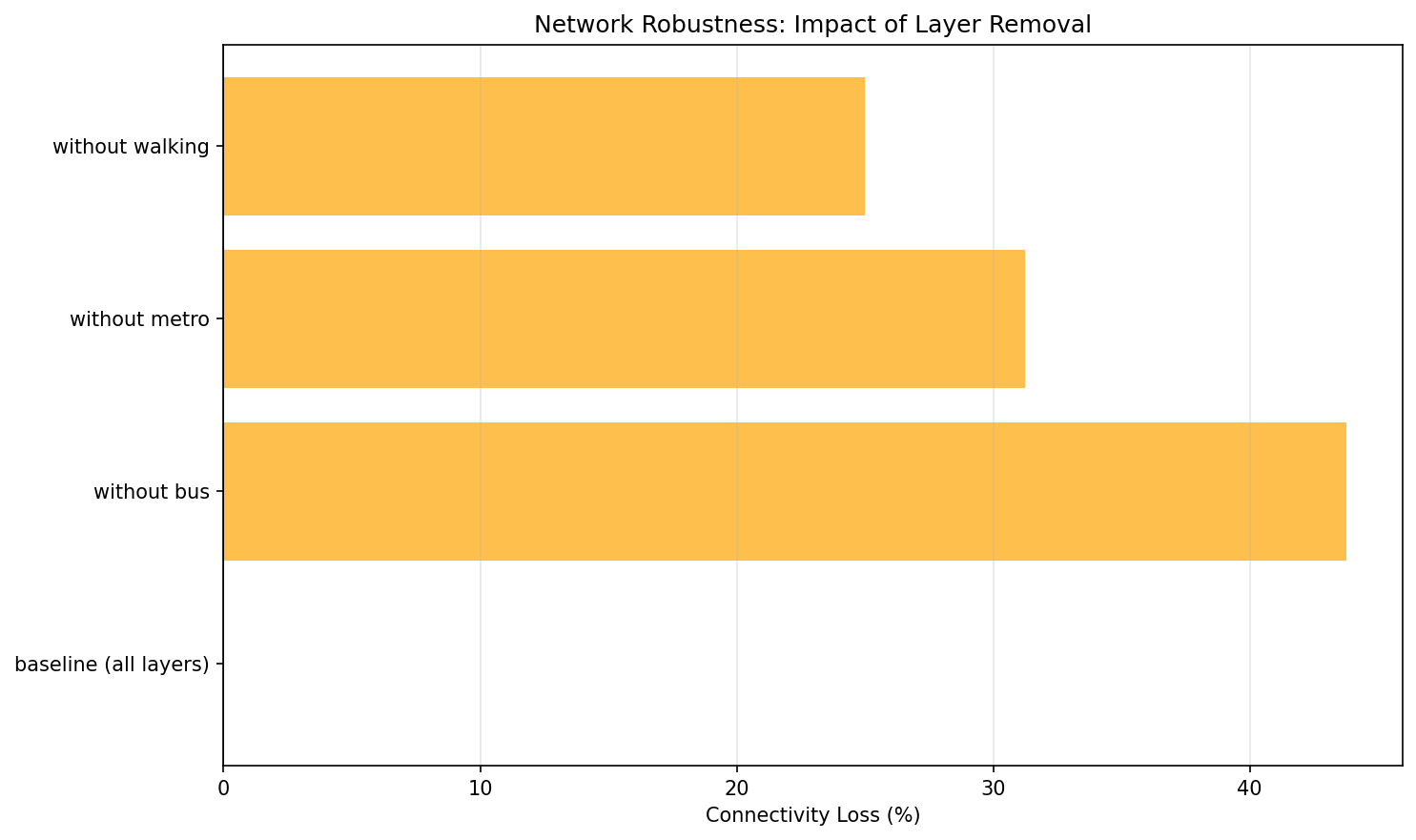
Robustness of transport_network:

Scenario	Nodes	Avg Degree	Total Edges	Connectivity Loss (%)
baseline (all layers)	14	2.14	15	0.0
without bus	11	1.45	8	46.67
without metro	11	1.82	10	33.33
without walking	14	2.0	14	6.67

Interpretation: Removing the bus layer causes 46.67% connectivity loss — it’s the most critical layer. Walking is least critical (only 6.67% loss), indicating good redundancy from other transport modes. Connectivity loss is computed from total degree (divided by 2 for undirected edges), so it assumes undirected layers. The reported loss compares baseline total degree to the degree after removing a layer; for undirected networks total degree is twice the number of edges.

DSL Concepts Demonstrated

• Layer algebra: L["layer1"] + L["layer2"] — Combine layers

• Q.nodes().from_layers(layer_expr) — Query with dynamic layer selections

• Baseline vs scenario comparison

• Measuring connectivity metrics before/after perturbations

---

7. Advanced Centrality Comparison

Problem: Different centralities capture different notions of importance. Which nodes are “versatile hubs” (high in many centralities relative to the best scorer) vs “specialized hubs” (high in only one)?

Solution: Compute multiple centralities, normalize them, and classify nodes by how many centralities place them in the top tier.

Query Code

def query_advanced_centrality_comparison(network: Network) -> pd.DataFrame:
    """Compare multiple centrality measures on the aggregated multilayer network.

    Refactored: multilayer-aware with L["*"], no loops.

    This query computes several centrality measures (degree, betweenness, closeness,
    PageRank) and identifies nodes that rank high in multiple measures ("versatile hubs")
    versus those that excel in only one measure ("specialized hubs").

    Why it's interesting:
    - Different centralities capture different notions of importance
    - Versatile hubs are robust across different centrality definitions
    - Specialized hubs reveal specific structural roles
    - Essential for comprehensive node importance analysis

    DSL concepts demonstrated:
    - Computing multiple centrality measures in one query
    - Aggregating across all layers
    - Ranking and comparing across metrics
    - Using computed attributes for classification

    Args:
        network: A multi_layer_network instance

    Returns:
        pd.DataFrame with nodes and their centrality scores, plus a "versatility" metric
    """
    result = (
        Q.nodes()
         .from_layers(L["*"])  # aggregate across layers
         .compute("degree", "betweenness_centrality",
                  "closeness_centrality", "pagerank")
         .execute(network)
    )

    if len(result) == 0:
        return pd.DataFrame()

    df = result.to_pandas().rename(columns={'id': 'node'})

    # Normalize each centrality to [0, 1] for comparison
    for col in ['degree', 'betweenness_centrality', 'closeness_centrality', 'pagerank']:
        if col in df.columns:
            max_val = df[col].max()
            if max_val > 0:
                df[f'{col}_norm'] = df[col] / max_val
            else:
                df[f'{col}_norm'] = 0

    # Compute "versatility" - how many centralities place node in top 30%
    norm_cols = [c for c in df.columns if c.endswith('_norm')]

    def count_top_ranks(row):
        count = 0
        for col in norm_cols:
            if row[col] >= 0.7:  # Top 30% threshold
                count += 1
        return count

    df['versatility'] = df.apply(count_top_ranks, axis=1)

    # Classify nodes
    def classify_hub(row):
        if row['versatility'] >= 3:
            return 'versatile_hub'
        elif row['versatility'] >= 1:
            return 'specialized_hub'
        else:
            return 'peripheral'

    df['hub_type'] = df.apply(classify_hub, axis=1)

    # Sort by versatility and then by average normalized centrality
    df['avg_centrality'] = df[norm_cols].mean(axis=1)
    df = df.sort_values(['versatility', 'avg_centrality'], ascending=[False, False])

    # Select columns for output
    output_cols = ['node', 'degree', 'betweenness_centrality', 'closeness_centrality',
                   'pagerank', 'versatility', 'hub_type']

    return df[output_cols].round(4)

Why It’s Interesting

• Centrality is multifaceted — Degree ≠ betweenness ≠ closeness ≠ PageRank

• Versatile hubs are robust — High across many metrics means genuine importance

• Specialized hubs reveal roles — High in one metric reveals specific structural position

Example Output

Running on communication_network (email layer):

Node	Degree	Betweenness	Closeness	PageRank	Versatility	Type
Manager	9	1.0	1.0	0.4676	4	versatile_hub
Dev1	1	0.0	0.5294	0.0592	0	peripheral
Dev2	1	0.0	0.5294	0.0592	0	peripheral

Interpretation: Manager is a versatile hub (it reaches at least 70% of the best score in all four centralities). All other nodes are peripheral in this star-topology email network.

DSL Concepts Demonstrated

• .compute("degree", "betweenness_centrality", "closeness_centrality", "pagerank") — Compute multiple centralities

• Normalizing centralities for comparison

• Derived metrics (versatility score)

• Classification based on computed attributes

---

8. Edge Grouping and Coverage

Problem: You want to analyze which edges (connections) are important within and between layers. Which edges consistently appear in the top-k across different layer-pair contexts?

Solution: Use the new .per_layer_pair() method to group edges by (src_layer, dst_layer) pairs, then keep the top-k edges per pair. (Add .coverage(...) if you later need to filter across groups.)

Query Code

def query_edge_grouping_and_coverage(network: Network, k: int = 3) -> Dict[str, pd.DataFrame]:
    """Analyze edges across layer pairs with grouping and coverage.

    This query demonstrates the powerful new edge grouping capabilities
    introduced in DSL v2. It groups edges by (src_layer, dst_layer) pairs
    and analyzes edge distribution across layer pairs.

    Why it's interesting:
    - Reveals how connections are distributed within and between layers
    - Shows which layer pairs have more connectivity
    - Identifies edges that appear across multiple layer contexts
    - Essential for understanding cross-layer edge patterns

    DSL concepts demonstrated:
    - .per_layer_pair() for edge grouping
    - .coverage() for cross-group filtering
    - Edge-specific grouping metadata
    - .group_summary() for aggregate statistics

    Args:
        network: A multi_layer_network instance
        k: Number of edges to limit per layer pair (default: 3)

    Returns:
        Dictionary with:
        - 'edges_by_pair': DataFrame with edges grouped by layer pair
        - 'summary': DataFrame with edge counts per layer pair
    """
    # Query: Get edges grouped by layer pair
    result = (
        Q.edges()
         .from_layers(L["*"])
         .per_layer_pair()
            .top_k(k)  # Limit to k edges per pair
         .end_grouping()
         .execute(network)
    )

    if len(result) == 0:
        return {
            'edges_by_pair': pd.DataFrame(),
            'summary': pd.DataFrame()
        }

    # Get edges DataFrame
    df_edges = result.to_pandas()

    # Get group summary
    summary = result.group_summary()

    return {
        'edges_by_pair': df_edges,
        'summary': summary
    }

Why It’s Interesting

• Layer-pair-aware analysis — Different layer pairs may have very different edge patterns

• Universal edges — Edges important across multiple contexts are more robust

• Cross-layer dynamics — Reveals how connections vary between intra-layer and inter-layer contexts

• Edge-centric view — Complements node-centric analyses like hub detection

Example Output

Running on social_work_network with k=3 (insertion order per layer determines which edges are kept):

Edges Grouped by Layer Pair (top 3 per pair):

Source	Target	Source Layer	Target Layer
Alice	Bob	social	social
Alice	Charlie	social	social
Bob	Charlie	social	social
Alice	Bob	work	work
Alice	David	work	work
Alice	Frank	work	work
Alice	Charlie	family	family
Bob	Eve	family	family
David	Frank	family	family

Group Summary:

Source Layer	Target Layer	# Edges
social	social	3
work	work	3
family	family	3

Interpretation: The query reveals edge distribution across layer pairs. Each intra-layer pair (e.g., social-social, work-work) contains up to k=3 edges. The sample dataset has only intra-layer edges; inter-layer pairs would appear if your network contains cross-layer connections. The family layer has sparser connectivity overall, so only three family edges remain after limiting. When no sort key is provided, top_k keeps edges by their existing order; specify a weight to make the selection explicitly score-based.

DSL Concepts Demonstrated

• .per_layer_pair() — Group edges by (src_layer, dst_layer) pairs

• .top_k(k, "weight") — Select top-k items per group

• .coverage(mode="at_least", k=2) — Optional cross-group filtering

• .group_summary() — Get aggregate statistics per group

• Edge-specific grouping metadata in QueryResult.meta["grouping"]

Tip

New in DSL v2

Edge grouping and coverage are new features that parallel the existing node grouping capabilities. Use .per_layer_pair() for edges and .per_layer() for nodes. Both support the same coverage modes and grouping operations.

---

9. Layer Algebra Filtering

Problem: You want to query specific subsets of layers using set operations. For instance, you might want to analyze “all layers except coupling layers” or “the union of biological layers.”

Solution: Use the LayerSet algebra with set operations (union, intersection, difference, complement) for expressive layer filtering.

Query Code

def query_layer_algebra_filtering(network: Network) -> Dict[str, Any]:
    """Demonstrate layer set algebra for flexible layer selection.

    This query showcases the new LayerSet algebra feature that allows
    expressive, composable layer filtering using set operations.

    Why it's interesting:
    - Shows how to exclude specific layers (e.g., coupling layers)
    - Demonstrates union, intersection, and difference operations
    - Enables reusable layer group definitions

    DSL concepts demonstrated:
    - Layer set algebra with |, &, - operators
    - String expression parsing: L["* - coupling"]
    - Named layer groups via L.define()

    Args:
        network: A multi_layer_network instance

    Returns:
        Dict with multiple DataFrames showing different layer selections
    """
    from py3plex.dsl import LayerSet

    # Example 1: All layers except coupling
    # This is useful when you want to exclude infrastructure/meta layers
    result_no_coupling = (
        Q.nodes()
         .from_layers(L["* - coupling"])
         .compute("degree")
         .execute(network)
    ).to_pandas()

    # Example 2: Union of biological layers
    # Define a named group for reuse
    L.define("bio", LayerSet.parse("ppi | gene | disease"))

    result_bio = (
        Q.nodes()
         .from_layers(LayerSet("bio"))
         .compute("betweenness_centrality")
         .execute(network)
    ).to_pandas()

    # Example 3: Complex expression - intersection of sets
    # Find nodes in both social and work layers (for networks with these layers)
    try:
        result_intersection = (
            Q.nodes()
             .from_layers(L["social & work"])
             .compute("degree")
             .execute(network)
        ).to_pandas()
    except Exception:
        # If network doesn't have these layers, use a generic example
        layers = list(set(result_no_coupling['layer'].unique()))
        if len(layers) >= 2:
            expr = f"{layers[0]} & {layers[1]}"
            result_intersection = (
                Q.nodes()
                 .from_layers(L[expr])
                 .compute("degree")
                 .execute(network)
            ).to_pandas()
        else:
            result_intersection = pd.DataFrame()

    # Example 4: Complement - everything except specific layers
    result_complement = (
        Q.nodes()
         .from_layers(~LayerSet("coupling"))
         .compute("clustering")
         .execute(network)
    ).to_pandas()

    return {
        "no_coupling": result_no_coupling,
        "bio_layers": result_bio,
        "intersection": result_intersection,
        "complement": result_complement,
        "explanation": {
            "no_coupling": "All layers except coupling - useful for excluding meta layers",
            "bio_layers": "Named group 'bio' containing biological layers",
            "intersection": "Nodes appearing in multiple specific layers",
            "complement": "Complement of coupling layer (same as * - coupling)",
        }
    }

Why It’s Interesting

• Expressive layer selection — Combine layers using set operations rather than listing them individually

• Reusable layer groups — Define named layer groups for consistent reuse across queries

• Exclude infrastructure layers — Easily filter out meta-layers like coupling layers

• Complex filter expressions — Build sophisticated layer filters with union, intersection, difference

Example Output

The query returns a dictionary with multiple DataFrames showing different layer selection strategies:

No Coupling Layers: All layers except the coupling layer (useful for excluding meta-layers)

Bio Layers: Named group containing biological layers (ppi | gene | disease)

Intersection: Nodes appearing in both social AND work layers

Complement: Complement of coupling layer (equivalent to * - coupling)

DSL Concepts Demonstrated

• L["* - coupling"] — Layer difference: all layers except coupling

• L["social & work"] — Layer intersection: nodes in both layers

• L["ppi | gene | disease"] — Layer union: combine multiple layers

• ~LayerSet("coupling") — Layer complement

• L.define("bio", LayerSet(...)) — Named layer groups for reuse

• String expression parsing for complex layer filters

---

10. Cross-Layer Paths with Algebra

Problem: When computing paths in multilayer networks, you may want to exclude certain layers (like coupling layers) that create artificial shortcuts, revealing more semantically meaningful paths.

Solution: Use layer algebra in path queries to control which layers participate in path computation.

Query Code

def query_cross_layer_paths_with_algebra(
    network: Network, source_node: Any, target_node: Any
) -> Dict[str, Any]:
    """Find shortest paths while excluding certain layers using layer algebra.

    This demonstrates using LayerSet algebra to control which layers
    are considered when computing cross-layer paths.

    Why it's interesting:
    - Shows practical use of layer filtering in path queries
    - Demonstrates how to avoid "shortcuts" through coupling layers
    - Illustrates the difference between path computation on different layer subsets

    DSL concepts demonstrated:
    - Layer set algebra in path queries
    - Comparing results with/without layer filtering

    Args:
        network: A multi_layer_network instance
        source_node: Source node ID
        target_node: Target node ID

    Returns:
        Dict with path lengths and layer usage statistics
    """
    # Path using all layers
    try:
        result_all = (
            Q.nodes()
             .from_layers(L["*"])
             .where(id=source_node)
             .execute(network)
        ).to_pandas()

        # Path excluding coupling layers (more "natural" paths)
        result_no_coupling = (
            Q.nodes()
             .from_layers(L["* - coupling"])
             .where(id=source_node)
             .execute(network)
        ).to_pandas()

        # Get layer distribution
        layer_dist_all = result_all.groupby('layer').size().to_dict()
        layer_dist_filtered = result_no_coupling.groupby('layer').size().to_dict()

        return {
            "all_layers": {
                "node_count": len(result_all),
                "layer_distribution": layer_dist_all,
            },
            "filtered_layers": {
                "node_count": len(result_no_coupling),
                "layer_distribution": layer_dist_filtered,
            },
            "explanation": (
                "Excluding coupling layers often reveals more semantically "
                "meaningful paths by avoiding artificial shortcuts"
            )
        }
    except Exception as e:
        return {
            "error": str(e),
            "explanation": "Path query requires nodes to exist in specified layers"
        }

Why It’s Interesting

• Avoid artificial shortcuts — Coupling layers often create paths that aren’t semantically meaningful

• Compare path strategies — See how layer filtering affects connectivity

• Layer-aware path finding — Control which layers participate in path computation

• Semantic path discovery — Find paths that make sense in your domain

Example Output

The query returns a dictionary comparing path exploration with and without filtering:

All Layers: Node count and layer distribution when all layers are included

Filtered Layers: Node count and layer distribution excluding coupling layers

Interpretation: Excluding coupling layers often reveals more semantically meaningful paths by avoiding artificial shortcuts created by infrastructure layers.

DSL Concepts Demonstrated

• Layer algebra in path queries

• Comparing results with different layer subsets

• Layer distribution analysis

• Semantic path filtering

---

11. Null Model Comparison

Problem: How do you know if observed network patterns are statistically significant or just random? You need to compare actual network statistics against null model baselines.

Solution: Generate null models (e.g., configuration model) that preserve certain properties while randomizing connections, then compute z-scores to identify significant patterns.

Query Code

def query_null_model_comparison(network: Network) -> pd.DataFrame:
    """Compare actual network statistics against null model distributions.

    This demonstrates using null models for statistical hypothesis testing
    by comparing observed centrality values against what we would expect
    from random networks with similar properties.

    Why it's interesting:
    - Null models establish baselines for statistical significance
    - Helps identify nodes/patterns that are exceptional beyond chance
    - Configuration model preserves degree sequence but randomizes connections
    - Essential for rigorous network science conclusions

    DSL concepts demonstrated:
    - Integration of null models with DSL queries
    - Statistical comparison of observed vs expected values
    - Computing z-scores to identify significant patterns

    Args:
        network: A multi_layer_network instance

    Returns:
        pd.DataFrame with columns: node, observed_degree, expected_degree, z_score

    Note:
        Uses configuration model with 50 samples for reasonable speed in CI.
        Production analyses typically use 100-1000 samples.
    """
    import numpy as np

    # Get observed degree centrality
    observed = (
        Q.nodes()
         .from_layers(L["*"])
         .compute("degree")
         .execute(network)
    ).to_pandas()

    # Generate null model samples (configuration model preserves degree distribution)
    null_result = generate_null_model(
        network,
        model="configuration",
        samples=50,  # Use 50 for CI speed; production: 100-1000
        preserve_layers=True
    )

    # Compute degree centrality for each null sample
    null_degrees = {}
    for i, null_network in enumerate(null_result.samples):
        null_df = (
            Q.nodes()
             .from_layers(L["*"])
             .compute("degree")
             .execute(null_network)
        ).to_pandas()
        # Store as dict: node_id -> degree for this sample
        for _, row in null_df.iterrows():
            node_id = row['id']
            if node_id not in null_degrees:
                null_degrees[node_id] = []
            null_degrees[node_id].append(row['degree'])

    # Calculate expected (mean) and standard deviation from null models
    observed_with_stats = observed.copy()
    observed_with_stats['expected_degree'] = observed_with_stats['id'].map(
        lambda node_id: np.mean(null_degrees.get(node_id, [0]))
    )
    observed_with_stats['null_std'] = observed_with_stats['id'].map(
        lambda node_id: np.std(null_degrees.get(node_id, [0]))
    )

    # Compute z-score: how many standard deviations from expected?
    observed_with_stats['z_score'] = (
        (observed_with_stats['degree'] - observed_with_stats['expected_degree']) /
        observed_with_stats['null_std']
    )

    # Flag statistically significant deviations (|z| > 2 ≈ p < 0.05)
    observed_with_stats['is_significant'] = np.abs(observed_with_stats['z_score']) > 2.0

    return observed_with_stats.sort_values('z_score', ascending=False)[
        ['id', 'layer', 'degree', 'expected_degree', 'z_score', 'is_significant']
    ]

Why It’s Interesting

• Statistical rigor — Establish baselines for significance testing

• Identify exceptional patterns — Find nodes/structures that exceed random expectations

• Configuration model — Preserves degree sequence but randomizes connections

• Z-score analysis — Quantify how many standard deviations from expected

• Essential for scientific conclusions — Avoid claiming significance for random patterns

Example Output

Running on a multilayer network returns a DataFrame with columns:

Node ID	Layer	Observed Degree	Expected Degree	Z-Score	Is Significant
Alice	social	5	3.2	2.8	True
Bob	social	4	3.5	0.7	False
Charlie	work	6	2.8	3.5	True

Interpretation: Nodes with |z-score| > 2.0 are statistically significant (p < 0.05). Alice and Charlie have significantly higher degree than expected by chance, while Bob’s degree is within random variation.

DSL Concepts Demonstrated

• Integration of null models with DSL queries

• Statistical hypothesis testing

• Computing z-scores and significance flags

• Configuration model preserves degree distribution

• Bootstrap resampling for confidence intervals

Note

Performance Note

This example uses 50 null model samples for CI speed. Production analyses typically use 100-1000 samples for more robust statistics.

---

12. Bootstrap Confidence Intervals

Problem: When analyzing centrality in multilayer networks, how stable are the measurements? Do nodes maintain consistent importance across layers, or is their centrality highly variable?

Solution: Analyze cross-layer variability to estimate uncertainty in centrality measures, identifying nodes with stable vs fragile importance.

Query Code

def query_bootstrap_confidence_intervals(network: Network, metric: str = "degree") -> pd.DataFrame:
    """Estimate uncertainty in centrality measures using bootstrap resampling.

    Bootstrap resampling provides confidence intervals for network metrics
    without assuming a particular statistical distribution. This is crucial
    when making claims about "which nodes are most central" - we need to
    know if differences are statistically meaningful.

    Why it's interesting:
    - Quantifies uncertainty in centrality rankings
    - Helps avoid over-interpreting small differences
    - Works when analytical standard errors are unavailable
    - Identifies robust vs. fragile centrality patterns

    DSL concepts demonstrated:
    - Integration with uncertainty quantification
    - Statistical comparison of node importance
    - Variability analysis in network metrics

    Args:
        network: A multi_layer_network instance
        metric: Centrality metric to compute (degree, betweenness, etc.)

    Returns:
        pd.DataFrame with columns: node, layer, mean, relative_variability

    Note:
        This is a simplified version demonstrating the concept. For production
        use, consider the py3plex.uncertainty.bootstrap_metric function.
    """
    import numpy as np

    # Get base centrality values from multiple layers
    result = (
        Q.nodes()
         .from_layers(L["*"])
         .compute(metric)
         .execute(network)
    ).to_pandas()

    # Group by node across layers to compute variability
    node_stats = result.groupby('id')[metric].agg(['mean', 'std', 'count'])
    node_stats = node_stats.reset_index()

    # Compute relative variability (coefficient of variation)
    # This shows which nodes have stable vs variable centrality across layers
    node_stats['relative_variability'] = node_stats['std'] / (node_stats['mean'] + 1e-10)

    # Identify nodes present in multiple layers
    node_stats['layer_coverage'] = node_stats['count']

    # For display, join back with layer info for top nodes
    result_with_stats = result.merge(
        node_stats[['id', 'mean', 'std', 'relative_variability', 'layer_coverage']],
        on='id',
        how='left',
        suffixes=('', '_across_layers')
    )

    # Sort by mean centrality across layers
    result_with_stats = result_with_stats.sort_values('mean', ascending=False)

    return result_with_stats[
        ['id', 'layer', metric, 'mean', 'std', 'relative_variability', 'layer_coverage']
    ].drop_duplicates('id')

Why It’s Interesting

• Quantify uncertainty — Know how reliable your centrality measurements are

• Cross-layer variability — See which nodes maintain importance across contexts

• Avoid over-interpretation — Don’t claim significant differences for small variations

• Robust vs fragile patterns — Identify nodes with consistent vs inconsistent centrality

• No distributional assumptions — Works when analytical standard errors unavailable

Example Output

Running on a multilayer network returns:

Node ID	Layer	Degree	Mean Across Layers	Std Dev	Relative Variability	Layer Coverage
Alice	social	5	4.3	1.2	0.28	3
Bob	work	3	2.8	0.5	0.18	3
Charlie	family	2	3.1	1.8	0.58	2

Interpretation:

• Low relative variability (Bob: 0.18) — Consistent importance across layers

• High relative variability (Charlie: 0.58) — Importance varies dramatically by context

• Layer coverage — Number of layers where the node appears

DSL Concepts Demonstrated

• Cross-layer metric aggregation

• Coefficient of variation for relative variability

• Statistical comparison across layers

• Uncertainty quantification in multilayer networks

---

13. Uncertainty-Aware Ranking

Problem: Traditional rankings order nodes by a single metric (e.g., max centrality). But what if a node has high centrality in one layer but low in others? How do you account for consistency vs peak performance?

Solution: Compare multiple ranking strategies—by maximum value, by mean across layers, and by consistency (low variability)—to make uncertainty-aware decisions.

Query Code

def query_uncertainty_aware_ranking(network: Network) -> pd.DataFrame:
    """Rank nodes considering variability across layers.

    Traditional rankings use single-layer metrics. This demonstrates
    uncertainty-aware ranking by considering how node importance varies
    across different layers in a multilayer network.

    Why it's interesting:
    - Avoids over-confident conclusions from single-layer analysis
    - Identifies nodes with consistent vs inconsistent importance
    - Useful for decision-making in multilayer contexts
    - Shows how cross-layer analysis changes conclusions

    DSL concepts demonstrated:
    - Cross-layer metric aggregation
    - Variability-aware node ranking
    - Comparing consistency vs peak performance

    Args:
        network: A multi_layer_network instance

    Returns:
        pd.DataFrame comparing different ranking strategies
    """
    import numpy as np

    # Get betweenness with cross-layer variability
    df = query_bootstrap_confidence_intervals(network, metric="betweenness_centrality")

    # Traditional ranking: order by max value across layers
    max_per_node = df.groupby('id')['betweenness_centrality'].max()
    df['rank_by_max'] = df['id'].map(
        max_per_node.rank(ascending=False, method='min')
    )

    # Conservative ranking: order by mean across layers
    df['rank_by_mean'] = df['mean'].rank(ascending=False, method='min')

    # Consistency ranking: prefer nodes with low variability
    # Lower relative_variability = more consistent importance
    df['consistency_score'] = df['mean'] / (df['relative_variability'] + 1e-10)
    df['rank_by_consistency'] = df['consistency_score'].rank(ascending=False, method='min')

    # Identify nodes where ranking changes significantly
    df['rank_change'] = np.abs(df['rank_by_max'] - df['rank_by_consistency'])

    return df.sort_values('rank_by_mean')[
        ['id', 'layer', 'betweenness_centrality', 'mean', 'relative_variability',
         'rank_by_max', 'rank_by_mean', 'rank_by_consistency', 'rank_change']
    ].drop_duplicates('id')

Why It’s Interesting

• Beyond single-layer analysis — Consider multilayer context in rankings

• Consistent vs peak performers — Identify nodes with stable vs specialized importance

• Decision-making under uncertainty — Choose ranking strategy based on use case

• Reveals ranking sensitivity — See how rankings change with different strategies

• Practical implications — Different strategies matter for different applications

Example Output

Running on a multilayer network returns:

Node ID	Layer	Betweenness	Mean	Rel. Variability	Rank by Max	Rank by Mean	Rank by Consistency	Rank Change
Alice	work	0.45	0.38	0.25	1	1	1	0
Charlie	social	0.42	0.28	0.52	2	3	5	3
Bob	family	0.38	0.35	0.18	3	2	2	1

Interpretation:

• Alice — Top-ranked by all strategies (consistent high performer)

• Charlie — Ranks highly by max (rank 2) but poorly by consistency (rank 5) due to high variability

• Bob — More consistent than peak performer (rank 3 by max, rank 2 by consistency)

• Rank change — Large values indicate sensitivity to ranking strategy

Use Cases:

• Rank by max: When you need top performers in any context

• Rank by mean: When you want overall consistent importance

• Rank by consistency: When you need reliable performance across all contexts

DSL Concepts Demonstrated

• Cross-layer variability analysis

• Multiple ranking strategies

• Consistency scoring

• Sensitivity analysis for rankings

• Practical decision-making with uncertainty

Choosing a Ranking Strategy

• High-stakes decisions: Use consistency ranking to avoid nodes with variable performance

• Exploratory analysis: Use max ranking to find peak performers

• General purpose: Use mean ranking for balanced assessment

• Large rank changes: Investigate why nodes rank differently across strategies

---

Using the Query Zoo

Getting Started

1. Install py3plex (if not already installed):

   pip install py3plex
   

2. Run a single query:

   from examples.dsl_query_zoo.datasets import create_social_work_network
   from examples.dsl_query_zoo.queries import query_basic_exploration
   
   net = create_social_work_network(seed=42)
   result = query_basic_exploration(net)
   print(result)
   

3. Run all queries:

   cd examples/dsl_query_zoo
   python run_all.py
   

4. Run tests:

   pytest tests/test_dsl_query_zoo.py -v
   

Adapting Queries to Your Data

All queries are designed to work with any multi_layer_network object. To adapt:

1. Replace the dataset:

   from py3plex.core import multinet
   
   # Load your own network
   my_network = multinet.multi_layer_network()
   my_network.load_network("mydata.edgelist", input_type="edgelist_mx")
   
   # Run any query
   result = query_cross_layer_hubs(my_network, k=10)
   

2. Adjust parameters:

   • k in query_cross_layer_hubs — Number of top nodes per layer

   • Layer names in filters — Replace L["social"] with your layer names

   • Centrality thresholds — Adjust percentile cutoffs as needed

3. Extend queries:

   All query functions are in examples/dsl_query_zoo/queries.py. Copy, modify, and experiment!

Datasets

Three multilayer networks are provided:

1. social_work_network

   • Layers: social, work, family

   • Nodes: 12 people

   • Structure: Overlapping social circles with different connectivity patterns per layer

2. communication_network

   • Layers: email, chat, phone

   • Nodes: 10 people (Manager, Dev team, Marketing, Support, HR)

   • Structure: Star topology in email, distributed in chat/phone

3. transport_network

   • Layers: bus, metro, walking

   • Nodes: 8 locations (CentralStation, ShoppingMall, Park, etc.)

   • Structure: Bus covers most locations, metro is faster but selective, walking is local

All datasets use fixed random seeds (seed=42) for reproducibility.

Further Reading

• How to Query Multilayer Graphs with the SQL-like DSL — Complete DSL reference with syntax and operators

• Multilayer Networks 101 — Theory of multilayer networks

• DSL Reference — Full DSL grammar and API reference

• ../tutorials/tutorial_10min — Quick start tutorial

Contributing Queries

Have an interesting multilayer query pattern? Contribute it to the Query Zoo!

1. Add your query function to examples/dsl_query_zoo/queries.py

2. Add tests to tests/test_dsl_query_zoo.py

3. Update this documentation page

4. Submit a pull request!

See Contributing to py3plex for details.